From the postbag Marjolein Hoekstra (CleverClogs) writes:
Short description
Can you make a Google Script for me that compares two strings character by character? If differences are found, the script should point these out. If no differences are found at all, the script should put out the text “[ id. ]” .
Detailed description
I have two columns containing lists of horizontally identical, but sometimes almost identical text strings. This is on purpose. Each row has another couple of words that need to be compared.
I’d like to compare them on a character by character basis, and then point out in the second column at which positions it differs from the first, for example like this:
A2: ABCDE
B2: ABKDE
If you compare these two, you’ll see that cell B2[3] has ‘K’ where A2[3] reads ‘C’.
My envisioned formula would then populate cell C2 with: “[ – – K – – ]”
As far as I can tell, I’d need a Google Script that parses both strings character by character and output “–” when they are identical, and output the value of the character string from B2. It should be relative simple, with a FOR loop. Thing is, I’ve never written a Google Script, and it’s a bit daunting for me to start on my own.
Note that LEN (A) is always identical to LEN (B)
Background info
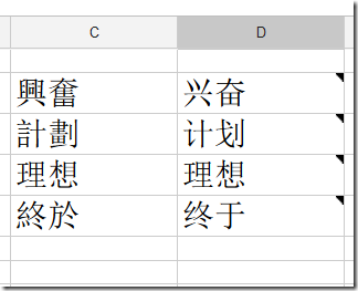
In case you’re interested in the actual use case: I want to use this formula to compare strings of Chinese characters, where the first column contains the traditional writing of these characters (typically requiring more strokes) and the second column containing the simplified writing of those same characters. Sometimes the characters are different, sometimes they are not. You can see this clearly in the screenshot below.
The Google Spreadsheet is used as input for a flashcard deck I’m building, using the iPhone app Flashcard Deluxe (top-notch system, highly flexible) [also available for Android].
Screenshot:


There’s no need to use Chinese characters to test the formula, I’m just providing this so that you know in what context the formula will be used.
The Solution
My initial thought was to use existing formula to SPLIT the cell text into individual character values and then do a comparison but unfortunately the SPLIT formula requires a character to split on. So instead I turned to Google Apps Script and wrote the following custom formula:
function stringComparison(s1, s2) {
  // lets test both variables are the same object type if not throw an error
  if (Object.prototype.toString.call(s1) !== Object.prototype.toString.call(s2)){
    throw("Both values need to be an array of cells or individual cells")
  }
  // if we are looking at two arrays of cells make sure the sizes match and only one column wide
  if( Object.prototype.toString.call(s1) === '[object Array]' ) {
    if (s1.length != s2.length || s1[0].length > 1 || s2[0].length > 1){
      throw("Arrays of cells need to be same size and 1 column wide");
    }
    // since we are working with an array intialise the return
    var out = [];
    for (r in s1){ // loop over the rows and find differences using diff sub function
      out.push([diff(s1[r][0], s2[r][0])]);
    }
    return out; // return response
  } else { // we are working with two cells so return diff
    return diff(s1, s2)
  }
}

function diff (s1, s2){
  var out = "[ ";
  var notid = false;
  // loop to match each character
  for (var n = 0; n < s1.length; n++){
    if (s1.charAt(n) == s2.charAt(n)){
      out += "–";
    } else {
      out += s2.charAt(n);
      notid = true;
    }
out += " ";
  }
  out += " ]"
  return (notid) ? out :  "[ id. ]"; // if notid(entical) return output or [id.]
}
One of the things to be aware of is Google Apps Script formulas are associated with a spreadsheet. You can’t globally use a custom formula unless the script is attached. Fortunately when copying a spreadsheet you also get a copy of the script, so providing templates is a way around this.
With this limitation in mind I thought I’d have another go at cracking this with built-in formula … and guess what it is possible. The key to unlocking this was when playing with the REGEXREPLACE formula I accidentally turned ‘ABCDE’ into ‘,A,B,C,D,E,’ by using =REGEXREPLACE(A20,"(.*?)",","). My RegEx is terrible so I’ll let someone else explain how this works in the comments, but getting to this point meant I could use a combination of SPLIT and REGEXREPLACE to do a character by character comparison on two cells of text. The final version of the formula goes (comparing cell A14 to B14):
=IF(EXACT(A14,B14),"[ id. ]","[ "&JOIN(" ",ARRAYFORMULA(REGEXREPLACE(SPLIT(REGEXREPLACE(B14,"(.*?)",","),","),SPLIT(REGEXREPLACE(A14,"(.*?)",","),","),"–")))&" ]")
My rough workings are embeded below. You can also make a copy of the entire project including the Apps Script solution here.
Update: Bruce Mcpherson has posted an alternative formula to do this which goes like:
"[ " & CONCATenate(ARRAYFORMULA(if(mid(A31, row(indirect("x1:x"&len(A31))) ,1)=mid(B31,row(indirect("x1:x"&len(A31))),1)," – "," "&mid(B31,row(indirect("x1:x"&len(A31)))&" ",1) ))) &" ]"
As you will see from the comments thread on that post Marjolein was having problems using my version with a Chinese characterset. Adding this to the example spreadsheet I’m unable to replicate the error but have encountered the problem here. If anyone can spot the difference I’d welcome your thoughts?
Update 2: Bruce pointed out that “the likely issue is that the columns with the problem are times – the characters mean AM. The same thing would probably happen with numbers. Have you tried wrapping the cell references in concatenate() to convert to a string?”
I said: ah I see what you mean 时 is being interpreted as 上午12:00:00. Not sure how I’d wrap the concatenate with my REGEXREPLACE. Your solution looks better all round so rather than loosing sleep I’d go with that
Google Spreadsheet: How to compare two strings ...
[…] How to compare two strings character by character in Google Spreadsheets using Google Apps Script or built-in Google Sheet formula […]