At the Association for Learning Technology (ALT) hosting large events is a regular activity and over the years we have developed bespoke workflows largely based in Google Sheets. In this post I’m going to share some of the tips we use for scheduling our events including drafting/publishing an event programme and how to keep in touch with your presenters.
These tips were presented at the free online ALT webinar How we run an online conference: ALT shares expertise on 09 April, 2020 which is going to be repeated on 29 April, 2020 at 3pm BST.
For some additional context ALT events are usually multi-strand covering 2-3 days and in terms of content there can be anything from 60 to 160 sessions in our programmes. For our events we usually do a double blind peer review. We manage the submission and peer review process in Google Sheets using a Google Apps Script powered workflow. The code for this has been published but it is far from ready for general public consumption, plus it needs refactoring for the new Google Apps Script runtime. In this post I’ll instead assume you have your speakers and sessions selected with basic programme information e.g. session title, theme, co-authors, lead author name and email etc. From this data I’ll show you the way we draft your programme and efficiently communicate with session leads.
As I know many of you find it easier to click around cells to see what is going on you can:
Copy ALT’s Programme Planning Template
Contents
- Tip #1: Unique session IDs
- Tip #2: VLOOKUP with defined arrays
- Tip #3: Use IMPORTRANGE to publish a copy of your draft programme
- Tip #4: Use prefilled Google Form fields and a mail merge for speaker communications
- Tip #5: ARRAYFORMULA can save lots of formula filling headaches
- Bonus Tip: Google Sheet charts are quick to style and easy to embed
- Summary
Tip #1: Unique session IDs
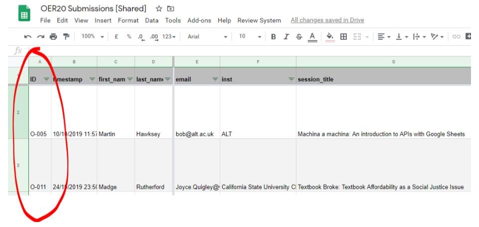
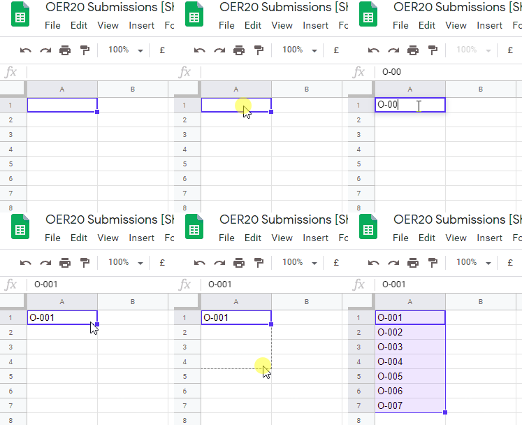
This might seem obvious but having a unique ID for all our sessions enables us to easily draft a programme and communicate with session leads. We generate our session IDs at the time of submission but Google Sheets is very good at filling down sequences:
Tip #2: VLOOKUP with defined arrays
We draft all our programmes in the same Google Sheet as our submissions. We’ve set up the grid we use to be similar to how the final programme is published on our website. Rather than copy/pasting session details like title and authors we use the VLOOKUP formula to pull this in based on the session IDs we use:
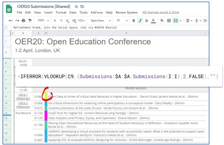
VLOOKUPIf you aren’t familiar with VLOOKUP the formula lets you search down the first column of a range for a key and returns the value of a specified cell in the row found. As our submission sheet has a lot of columns we also use { } brackets to select ranges that might not be next to each other (read more about using arrays in Google Sheets). We also use VLOOKUP to pull back where a session is timetabled into the main submission sheet so we can cross check if, when and where something is scheduled in the programme.
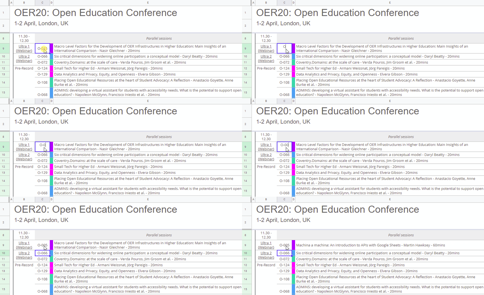
… in the case of session title, authors and duration we concatenate using multiple VLOOKUP in one formula:
=IFERROR(VLOOKUP(C9,{Submissions!$A:$A,Submissions!G:G},2,FALSE)
&" - "&VLOOKUP(C9,{Submissions!$A:$A,Submissions!$AT:$AT},2,FALSE)
&" - "&VLOOKUP(C9,{Submissions!$A:$A,Submissions!$AS:$AS},2,FALSE)
&"mins","")
Tip #3: Use IMPORTRANGE to publish a copy of your draft programme
If you’ve not used IMPORTRANGE before it’s a powerful formula that lets you include cells from another Google Sheet without sharing the entire spreadsheet. In the case of our events once we have drafted the programme in our main submission spreadsheet we use IMPORTRANGE to have a published version that automatically updates to changes in the draft. Our second Google Sheet can be shared with anyone without the fear of sharing too much personal information.
The steps we use to set this up is to copy our draft programme tab to a new Google Sheet so we also have a copy of all the formatting. Cell values are then removed from the copied version and IMPORTRANGE used to dynamically pull the values:
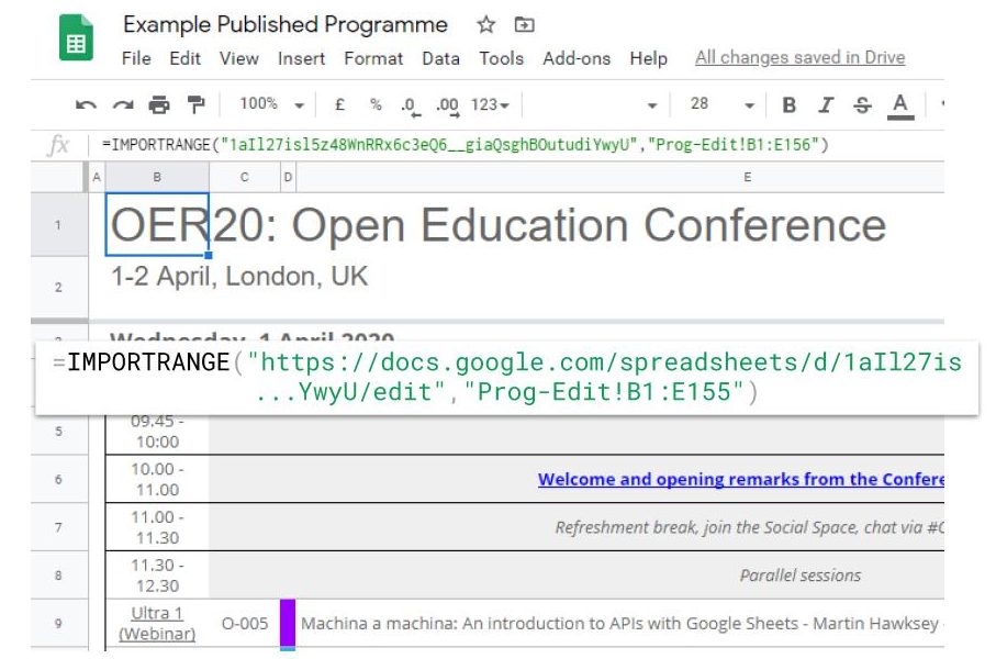
IMPORTRANGE to pull live data from a protected sheetTip #4: Use prefilled Google Form fields and a mail merge for speaker communications
Often for events we need additional bit of information from our session presenters. This might be managing media permissions or just checking the slot they’ve been scheduled in the programme is suitable. To simplify this process we often email presenters and include a link to a Google Form using links that have fields filled in with information like their session ID. As the Form responses have a session ID it also means we can automatically pull their responses into our master submission sheet.
To include a session ID in the email we send we also use a mail merge to send personal emails in bulk. Google doesn’t include a built-in mail merge tool within Google Sheets but there is a growing list of mail merge add-ons you can use … and for the more adventurous I’ve published a mail merge solution in the G Suite Developer Solutions Gallery (a modified version is included in the Programme Planning Template).
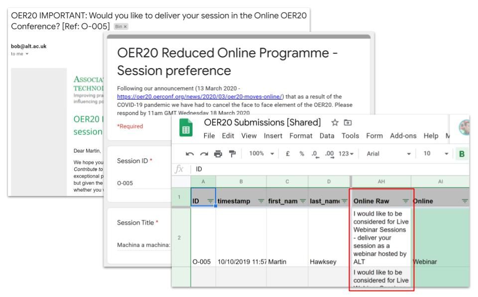
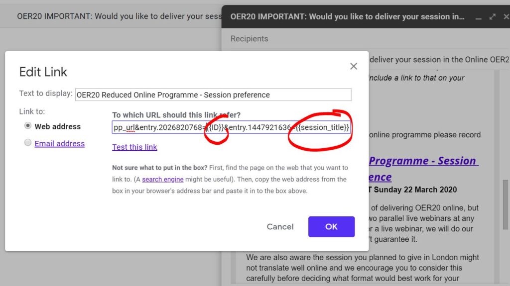
Update: Using pre-filled Google Form links with a mail merge depends on the solution you are using and how data is merged into your email. In the case of the shared ALT Programme Planning Template row values are identified by adding {{ }} around column heading names. Here’s an example of a pre-filled Google Form link setup for our Gmail mail merge where we include the speakers session ID and session title:
Tip #5: ARRAYFORMULA can save lots of formula filling headaches
Another trick we use extensively at ALT is ARRAYFORMULA. With ARRAYFORMULA we can write a formula once and then have it applied to an entire column, removing the need to copy/paste or fill down, also particularly useful when you might have new data coming in to a sheet from a Google Form.
This saves a lot of time but a note of caution – if you have a header row and put your ARRAYFORMULA in row 2 referencing the remainder of the column, if someone sorts the rows it might put your formula on a different row breaking your carefully crafted formula. This is why where possible we design our ARRAYFORMULA to go in the heading row using { } brackets and semicolons to specify a column header name and the ARRAYFORMULA.
Below is an example of where we pull speaker Google Form responses back into our main submission sheet and you can also see it in action here:
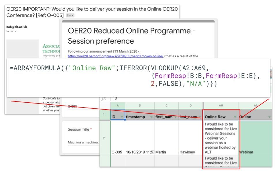
ARRAYFORMULABonus Tip: Google Sheet charts are quick to style and easy to embed
The charting abilities in Google Sheets have come a long way and as well as making it easier to design meaningful and attractive graphs these can also be embedded into other websites and update automatically when new data is added.
For example, when we recently had to cancel a face-to-face conference and move online we wanted to include a donations widget:
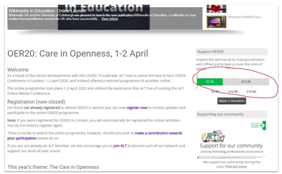
The widget uses a Google Sheet where we were able to record realtime data, automatically updating the bar graph we included in our site. If you’d like to do something similar you can copy our OER20 Donation Widget Google Sheet and follow the instructions.
Summary
This post has covered some of the regular tricks we use when planning event programmes with Google Sheets. Looking through ALT’s Programme Planning Template I’m sure you’ll find more examples of the way we both use and reshape data for our events. If you have any other examples similar to this or questions feel free to get in touch.